Indoor Positioning with Deep Learning: Turning Beacon Signals into Coordinates

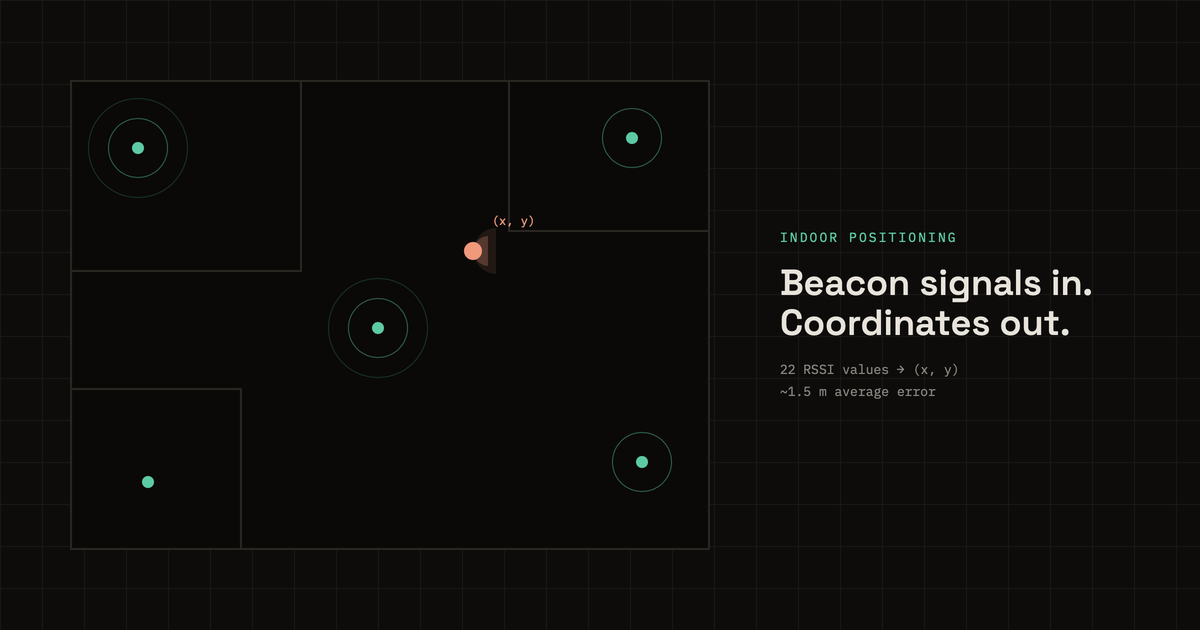
Imagine a floor full of desks, meeting rooms, and corridors, with small Bluetooth beacons mounted around it. Every beacon shouts a signal, and a phone or badge in someone’s pocket hears several of them at once, each at a different strength. From those signal strengths alone, we want to answer a deceptively hard question: where on the floor is this person standing?

Our system already had an answer, and it was the obvious one: whichever beacon the device hears loudest, assume the person is next to it. That “nearest beacon” method is simple and it works, until it doesn’t. Indoors, signal strength is noisy. Walls, furniture, bodies, and other radios all bend and weaken the signal, so the loudest beacon is often not the closest one. The estimate jumps around, and in a dense layout where beacons are only a few meters apart, being off by “one beacon” can put you in the wrong room.

This post is the engineering story of trying to do better with machine learning. It is not a step-by-step tutorial; it is the honest version, the problem, the approaches we tried, the two that failed, and the one that worked. By the end we had a small neural network that predicts a person’s (x, y) position on the floorplan directly from beacon signal strengths, and beats the nearest-beacon baseline on most of the test points.

Throughout, the beacon identifiers (MAC addresses) are fictitious. Substitute your own.

The problem

A beacon deployment looks like this: anchors placed across the floor so that, ideally, every spot hears at least a few of them.

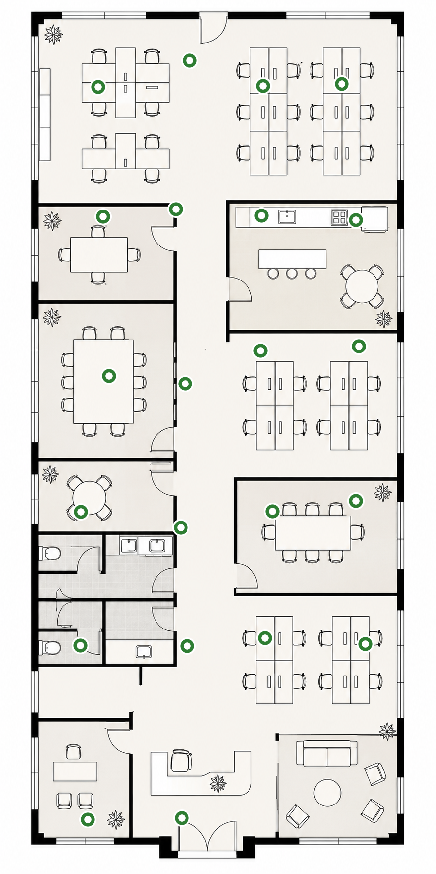
Each device continuously reports what it hears. A single reading is a list of anchors (the beacons in range) with an RSSI value for each, the Received Signal Strength Indicator, measured in dBm. RSSI is always negative, and closer to zero means stronger: -65 is a strong, nearby signal; -85 is weak and far. The catch is that “far” in dBm is not “far” in meters. Reflections and obstacles routinely make a beacon across the room read stronger than one right beside you.

The nearest-beacon method throws away almost all of this. It looks at the single strongest RSSI and ignores the rest. But the combination of signals carries far more information: hearing beacon A loud, B medium, and C faint is a fingerprint of a specific spot on the floor. The question was whether a model could learn to read that fingerprint and turn it into coordinates.

The data

We collected data over MQTT, the lightweight publish/subscribe protocol that IoT devices use. As a person stood at a known spot, the system logged every beacon the device heard, and we recorded that spot’s (x, y) position by marking it on the floorplan by hand. Each record pairs the raw beacon readings with the true location, which is exactly what a supervised model needs.

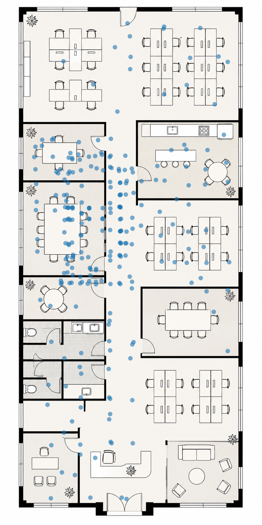
We gathered roughly 5,200 records. Training data was collected across the floor:

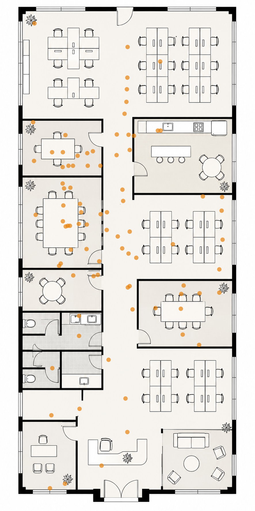
A portion of the points was held out as a test set, used only to score the finished model, never to train it:

A single raw record looks like this, a set of anchors with their RSSI, plus the ground-truth position:

{
  "anchors": [
    { "mac": "A1B2C3D4E5F6", "rssi": -65 },
    { "mac": "B2C3D4E5F6A1", "rssi": -66 },
    { "mac": "C3D4E5F6A1B2", "rssi": -71 },
    { "mac": "D4E5F6A1B2C3", "rssi": -73 },
    { "mac": "E5F6A1B2C3D4", "rssi": -76 }
  ],
  "params": { "x": 89.92, "y": 237.75 }
}

x and y are pixel coordinates on the floorplan image. That is what we want to predict.

The stack

There are two halves here with a clean line between them: the production platform that collects the data, and the Python pipeline that learns from it.

The collection side is serverless on AWS. Devices publish what they hear over MQTT to AWS IoT Core, and a set of Node/TypeScript Lambdas process each reading and persist it into PostgreSQL on Amazon RDS. For this project the stored readings, the anchors, their RSSI, and the hand-marked (x, y), were exported to JSON, so the modeling work reads flat files and never touches the live database.

The modeling side is plain Python, with a small set of well-worn libraries:

• Data wrangling: pandas + NumPy. Building the fixed 22-column table, grouping by location, and averaging readings is all pandas and NumPy.
• Modeling: PyTorch. The regression network, the training loop, and the custom Euclidean-distance loss are plain PyTorch.
• Scaling and splitting: scikit-learn. MinMaxScaler for normalization, train_test_split for the train/test division.
• Persistence: joblib. The trained weights and, just as importantly, the fitted scalers are saved with joblib so inference reproduces training exactly.
• Plots: matplotlib. The distance comparison and the diagnostic charts.

The approaches we took

Every data-science project has the same unglamorous first half: before you can compare models, you have to get the data into shape, clean it up, normalize it, and strip out the noise and redundancy that would mislead any model. Only then does the interesting question start: which model? We did not land on the regression network on the first try. We treated model choice as a real question and put three candidates against a single yardstick, does it place a person more accurately than the nearest-beacon method, and let two of them lose.

Cleaning up the data: de-dup, normalization, and features

Before any model, the raw readings had to become a fixed, clean, numeric table. This is the standard data-prep every project shares, cleanup, de-duplication, and normalization, and here it mattered more than the model choice did.

Every record must have the same columns. A model needs a fixed-width input, but each reading only contains the beacons that happened to be in range. So we fixed a list of the 22 relevant anchors and, for any beacon a reading did not hear, filled in a zero. Every record becomes a row with the same 22 beacon columns plus x and y.

Flip the RSSI to a positive “strength”. Raw RSSI is negative and awkward to reason about, so we converted each value to a positive number where bigger means stronger, and an absent beacon is a clean zero:

rssi = abs(anchors[anchor])   # -65 -> 65
rssi = 100 - rssi             # 65  -> 35   (stronger = higher)
# beacons not heard in this reading are filled with 0

So the raw record above becomes a flat row: the five heard beacons get strengths of 35, 34, 29, 27, and 24, and the other seventeen anchors are 0.

{
  "A1B2C3D4E5F6": 35, "B2C3D4E5F6A1": 34, "C3D4E5F6A1B2": 29,
  "D4E5F6A1B2C3": 27, "E5F6A1B2C3D4": 24, "F6A1B2C3D4E5": 0,
  "...": 0,
  "x": 89.92, "y": 237.75
}

Drop near-duplicate points. People stood in clusters, so many samples sat almost on top of each other and would bias the model toward crowded spots. We removed points that were closer than a threshold using plain Euclidean distance, keeping the collection spread out:

distance_threshold = 15

filter_points = []
for point in unique_points:
    if all(euclidean_distance(point, kept) >= distance_threshold for kept in filter_points):
        filter_points.append(point)

Average the readings per location. A spot was usually sampled several times, so for each location we averaged the strength of each beacon across its readings (ignoring the zeros, so an occasional miss did not drag a strong beacon down) and kept the most relevant anchors per point. This gave one clean, representative row per location.

Normalize. Finally, both the beacon strengths and the (x, y) coordinates were scaled to the [0, 1] range with Min-Max scaling, so no single feature dominates training. The scalers are saved so predictions can be converted back into real floorplan coordinates later.

scaler_beacons = MinMaxScaler()
beacons_normalized = scaler_beacons.fit_transform(beacons)

scaler_xy = MinMaxScaler()
xy_normalized = scaler_xy.fit_transform(x_y)

With the data in shape, we tried three models. The first two did not work, and it is worth saying why.

Attempt 1 — a GAN

Our first instinct was that 5,200 records is not a lot, and more data usually helps. A Generative Adversarial Network is the fashionable way to manufacture more: two networks trained against each other, a generator inventing synthetic samples and a discriminator trying to tell fake from real, until the fakes look convincing. The plan was to generate extra, realistic beacon-and-position samples to enrich the dataset.

It failed. The GAN never learned to spread its output across the floor; instead it collapsed the synthetic points into a tight blob that captured none of the variety of real positions.

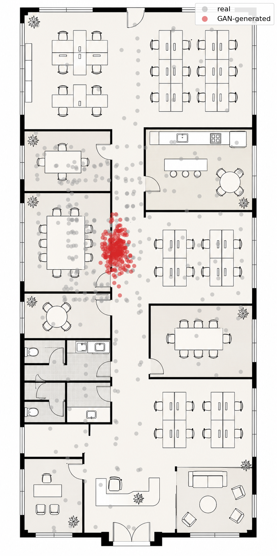
In hindsight this makes sense. GANs shine at generating images, audio, and text, where “realistic” is fuzzy and there is no single correct answer. Our problem is the opposite: it needs precise, numeric relationships between signal strengths and an exact coordinate. Synthetic points that are merely plausible do not help a task whose whole point is accuracy, and the classic failure mode of GANs, mode collapse, is exactly the blob we got. We set it aside.

Attempt 2 — an RNN

The data was collected in time order, one reading after another, so a Recurrent Neural Network looked tempting. RNNs are built for sequences: they carry information from earlier steps forward, which is powerful when the order of the data means something.

The problem is that the order in our data is an accident of collection, not a real signal. In production the model has to answer right now, from the current beacon readings, with no history to lean on. There is no sequence to feed it. Forcing one in during training added complexity and tuning pain without improving accuracy, because the thing that actually predicts position, the spatial relationship between signal strengths and coordinates, does not depend on what was measured a moment earlier. So the RNN went the way of the GAN.

What worked — a small regression network

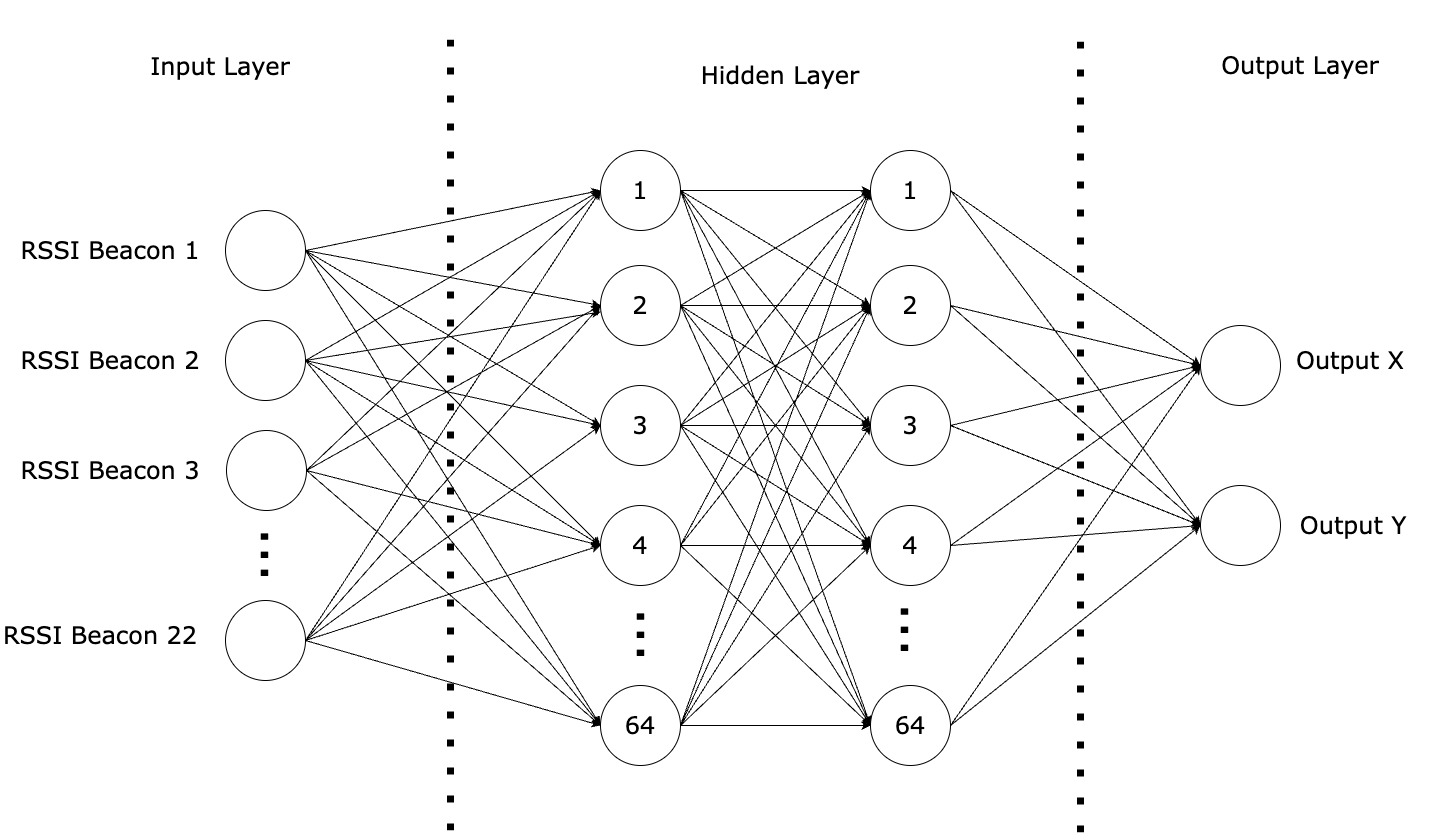
Stepping back from the fancy options, the task is plainly a regression: 22 numbers in (the beacon strengths), 2 numbers out (the x and y coordinates). So we built a small, ordinary feed-forward network in PyTorch to do exactly that. The rest of this section is the solution in full, because it is the part worth getting right: the architecture and why it is shaped this way, the loss that made it work, how training actually went, and how a single live reading turns into a dot on the map.

The architecture

The network has three parts, and it is deliberately small.

class BeaconNetwork(nn.Module):
    def __init__(self):
        super().__init__()
        self.common_layers = nn.Sequential(
            nn.Linear(22, 64),   # expand the 22 beacon strengths
            nn.LeakyReLU(),
            nn.Linear(64, 64),   # mix them into higher-level features
            nn.LeakyReLU(),
        )
        self.regression_head = nn.Linear(64, 2)  # distil down to (x, y)

    def forward(self, x):
        return self.regression_head(self.common_layers(x))

Reading it top to bottom:

• The input is 22 numbers, one per anchor in our fixed beacon list, each a signal strength (or zero if that beacon was not heard). This is the fingerprint of a location.
• The common layers widen 22 into 64, then keep it at 64. Widening gives the network room to learn combinations, “A loud and C faint means the north corridor” is a pattern that a single raw input cannot express but a 64-dimensional hidden layer can. The second 64-unit layer lets it compose those patterns into higher-level ones. Two layers were enough; going deeper on 5,200 records only invited overfitting for no accuracy gain.
• Between the layers we use LeakyReLU instead of a plain ReLU. A plain ReLU outputs zero for any negative input, and a unit that gets stuck outputting zero stops learning entirely (its gradient is zero, so training can never revive it, the “dying ReLU” problem). LeakyReLU leaks a small slope for negatives, so every unit keeps a little gradient and keeps learning. With a small network where we cannot afford to waste units, that matters.
• The regression head collapses the 64 features to exactly two numbers: the predicted x and y. No activation on the output, because coordinates are unbounded values, not probabilities.

That is the whole model. It has a few thousand parameters and trains in seconds on a laptop.

It helps to picture what those hidden layers are actually doing. The nearest-beacon method looks at a single number, the strongest signal, and discards everything else. This network looks at all 22 strengths at once and learns which patterns of loud-and-faint correspond to which part of the floor. Two spots that share the same loudest beacon but differ in the quieter ones behind it, the exact case the old method confuses, land in different places here, because the hidden layers encode the whole shape of the signal, not just its peak. That is the entire reason a model helps: the information about position was always in the combination of signals, and this network is simply the thing that finally reads it. Its small size is a feature, not a compromise. There is only so much to learn from 22 inputs and a few thousand locations, and a bigger network would memorize the training points instead of generalizing between them.

Matching the loss to the goal

The single most important decision was not the architecture, it was the loss function.

The obvious choice for regression is mean squared error, which would optimize x and y independently. But we do not care about x and y on their own, we care about how far the predicted dot lands from the real one. Those are not the same thing: a model can have a small error on x and a small error on y and still put the dot in the wrong place. So we trained the network directly on the Euclidean distance between the predicted and true location, the exact quantity a user would measure with a ruler on the floorplan:

def euclidean_distance_loss(output, target):
    # straight-line distance per sample, averaged over the batch
    return torch.sqrt(torch.sum((output - target) ** 2, dim=1)).mean()

Optimizing this means every training step nudges the network to shrink the actual gap between guess and truth. The objective and the metric we report are the same number, so there is no gap between “what we trained for” and “what we measure.”

Training

Training was deliberately unremarkable, and that was the point: no exotic schedule, no hand-tuned learning rate. We used the Adam optimizer with its defaults and ran 150 passes over the data, backpropagating the Euclidean-distance loss on every step. The average distance loss (in normalized [0, 1] units) fell steadily and was still improving gently at the end rather than thrashing, which is the signature of a network learning real structure instead of memorizing points:

Epoch   1, avg loss: 0.2253
Epoch  10, avg loss: 0.1185
Epoch  50, avg loss: 0.0825
Epoch 100, avg loss: 0.0710
Epoch 150, avg loss: 0.0583

One decision here is easy to overlook but is genuinely part of the model: we saved the Min-Max scalers alongside the weights. A prediction comes out in normalized space, and only the exact scalers fit during training can map a raw reading into the network’s input range and map its output back into real floorplan pixels. The weights and the two scalers are one indivisible artifact, ship the weights alone and the model is useless.

From signals to a point on the map

The payoff is a clean, fast path from a live reading to a dot on the floorplan, and it is simply the preprocessing run forward and then undone at the end:

1. Assemble the 22-length input from the current reading, with the same fixed anchor list and the same 100 - |rssi| transform, zero-filling any beacon not heard. The live input has to be built exactly the way the training rows were, or the network sees a distribution it never learned.
2. Normalize it with the saved beacon scaler, never a fresh one fit on the single reading.
3. Forward pass in inference mode (model.eval() with gradients off) to get a normalized (x, y) quickly and deterministically.
4. Inverse-transform with the saved xy scaler to land back on real floorplan pixels.

The result is an (x, y) you can draw straight onto the floorplan, one dot placed from the whole chord of beacon signals rather than the loudest note. And because the network is only a few thousand parameters, that entire path runs in milliseconds on modest hardware, no GPU, no cloud round-trip, which for a system that has to answer continuously matters as much as the accuracy does.

Results

To evaluate, we ran the trained model on the test points, converted the predictions back from normalized values into real floorplan coordinates with the saved scaler, and measured the Euclidean distance between each prediction and the true position. On the floorplan that average error is about 15 units, and units on a plan mean nothing to a reader. On the real office floor this was collected on, it works out to about 1.5 meters of average error, close enough to place someone in the right room or work zone, which is exactly the resolution the nearest-beacon method kept getting wrong.

The number that matters is the comparison against the method we set out to beat. The nearest-beacon method is the control here, the existing baseline, and the model has to beat it on the very same held-out points. For each test point we measured two distances: how far the model’s prediction landed from the truth, and how far the nearest beacon was. Sorted from best to worst, the model’s error (blue) sits below the nearest-beacon error (orange) across most of the range:

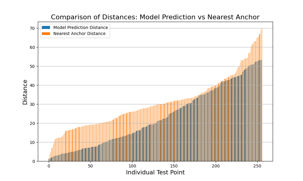
The model is not perfect, and at the hardest points, corners and dead zones where few beacons are heard, both methods struggle. But across the floor it consistently lands closer to the truth than the nearest-beacon baseline, which means it is genuinely reading the combination of signals rather than just the loudest one.

What we learned

The headline is almost anticlimactic: the simplest model won. The GAN and the RNN were the interesting ideas, and both were the wrong tool. The GAN was solving a problem we did not have (generating plausible variety) for a task that needs the opposite (numeric precision). The RNN was exploiting an order that would not exist at inference time. A plain regression network, pointed at the right objective, beat both without drama.

A few things carried the result more than the model choice did:

• The features did the heavy lifting. Fixing a consistent set of anchors, zero-filling missing beacons, flipping RSSI into a positive strength, de-duplicating crowded points, and averaging per location mattered more than any architecture tweak.
• Match the loss to the goal. Training on Euclidean distance instead of a generic per-coordinate loss meant the network optimized the exact thing we cared about.
• Reach for the fancy model last. GANs and RNNs are powerful, but “powerful” is not “suitable.” Naming the task honestly, this is regression, pointed us at the model that actually fit.

Beacon-based location does not have to mean “whichever one is loudest.” With a modest amount of labeled data and a small network trained on the right objective, the combination of signals is enough to place someone on a floorplan more accurately than proximity alone, and the whole thing is small enough to run anywhere.