RF Filter Design for ESP32-S3, Part 4: Track Keepout and Crosstalk Isolation
In this post, we demonstrate why traces routed beneath an RF path degrade an ESP32-S3 filter even when the schematic says they’re isolated, and how Track Keepout in Altium, CST re-simulation and component re-tuning restore isolation without giving up S₁₁ matching.


Eliminating parasitic coupling through controlled routing exclusion zones
"Crosstalk is not a defect of the circuit; it is a consequence of treating the layout as invisible."
— Henry Ott, Electromagnetic Compatibility Engineering (2009)
Introduction
The preceding three articles established a complete electrical and electromagnetic baseline for an RF filter designed for the ESP32-S3 Wi-Fi system. Article 1 defined an ideal CLC topology and optimized it in the schematic domain. Article 2 imported the PCB layout into CST Studio Suite, revealing how physical routing geometry affects the filter response. Article 3 replaced ideal component models with real manufacturer datasheets from Murata, bringing the simulation to a level of accuracy that reflects actual hardware behavior.
At the conclusion of Article 3, the filter design had achieved excellent matching across the target frequency band (2402–2480 MHz), with S1,1 values ranging from −15.31 dB to −26.34 dB, well within specifications. The component values had been optimized specifically for the layout environment in which they would operate. The simulation matched the physics of the board.
However, the design remained incomplete in one critical dimension: electromagnetic isolation. The PCB layout revealed a structural problem that simulation alone could not address: signal traces carrying digital control lines, power distribution, and clock signals passed directly beneath the RF filter trace on internal layers. These traces, while electrically isolated from the RF path, created parasitic coupling paths through capacitive and inductive effects. The E-field and H-field visualizations from the full-wave simulation showed energy concentration not only at the RF nodes but also in the dielectric layers below, indicating that crosstalk energy was being coupled to adjacent signal paths.
This is the classic multilayer RF problem: isolation and immunity cannot be solved by component selection alone. They require modification of the physical routing environment, specifically, the exclusion of interfering signals from the space directly adjacent to critical RF traces.
Track Keepout is a routing constraint tool in Altium Designer that creates zones where certain classes of routing are prohibited. Unlike copper removal, which modifies the stackup and changes impedance characteristics, a Track Keepout restriction preserves the ground plane structure while preventing signal traces from occupying specific regions. This distinction is essential: the goal is not to remove copper, but to enforce a "no signal traces" discipline in a defined area.
This article documents the practical implementation of Track Keepout polygons in the ESP32-S3 filter layout, the electromagnetic effects observed in CST simulation, and the component re-optimization required to account for the changed impedance environment created by the exclusion zone. The initial implementation of Track Keepout, without component adjustment, degraded performance significantly: S1,1 at 2462 MHz dropped to −19.10 dB (a +7.24 dB degradation from the baseline −26.34 dB). Subsequent component re-optimization recovered most of that loss, bringing 2462 MHz to −22.37 dB (a residual +3.97 dB degradation). At 2402 and 2437 MHz, the optimized design actually exceeds baseline performance, achieving −15.75 dB and −22.46 dB respectively, improvements of −0.44 dB and −0.32 dB over baseline.
It demonstrates a workflow in which crosstalk mitigation is achieved iteratively: first by isolation technique (Track Keepout), then by validation through full-wave simulation, then by component adjustment to maintain performance.
The result is a design in which electromagnetic confinement is achieved without sacrificing RF matching, a necessary foundation for the advanced mitigation techniques (via stitching and ground plane control) that follow in Articles 5 and 6.
The Problem: Crosstalk in Multilayer PCB
Multilayer Architecture and Signal Proximity
Modern RF PCBs for IoT and embedded systems are constrained by size, cost, and thermal management requirements. A four-layer stackup is the practical minimum for such designs:
- Layer 1 (Top): RF signal traces, component pads, vias
- Layer 2 (Mid-1): Mixed-signal routing, clock lines, control signals, power distribution
- Layer 3 (Mid-2): Ground plane with strategic apertures for signal routing
- Layer 4 (Bottom): Return paths, additional signal routing, power planes
In the ESP32-S3 reference design, the RF filter circuit occupies a region approximately 15 mm × 8 mm on Layer 1. The three RF components, the two capacitors (CRF1, CRF2) and the series inductor (R0L), are arranged in a tight PI configuration to minimize trace length and parasitic inductance.
However, directly beneath this RF zone on Layer 2 lie several signal traces that serve the digital subsystem: a clock line driving the SPI interface, a control signal for the RF switch, and distributed power lines. These traces do not share any direct electrical connection with the RF filter circuit. They are routed on a different layer, referenced to a different ground plane segment, and terminated on different receiver nodes. From a circuit schematic perspective, they are completely isolated.
From an electromagnetic perspective, they are catastrophically coupled.
Parasitic Coupling Mechanisms
The coupling between the RF trace on Layer 1 and the interfering traces on Layer 2 occurs through two primary mechanisms:
Capacitive Coupling: The copper conductor on Layer 1 and the copper conductor on Layer 2 are separated by a thin dielectric (the stackup dielectric immediately beneath Layer 1). This separation forms a distributed capacitor:
C = ε₀ × εᵣ × A / dwhere A is the area of geometric overlap and d is the separation distance.
Inductive Coupling: The two traces also form a distributed transformer through their mutual inductance. A current transient on the Layer 2 trace induces a magnetic field that threads the loop formed by the Layer 1 trace and its return path. This effect is frequency-dependent and most pronounced near the loop's resonant frequency.
Together, these mechanisms create a parasitic network that modifies the effective impedance at the input of the RF filter. Instead of the filter seeing a clean 35 Ω source, it sees an impedance that varies with frequency and with the switching activity on the nearby digital lines.
PCB Stackup and Layer Separation
The actual PCB stackup for the ESP32-S3 design consists of the following layers:
| Layer | Name | Material | Type | Thickness | Dielectric Constant |
|---|---|---|---|---|---|
| 1 | Top Layer | — | Signal | 0.0359 mm | — |
| — | Dielectric 1 | FR-4 | Dielectric | 0.2104 mm | 4.4 |
| 2 | Mid-Layer 1 | — | Signal | 0.0152 mm | — |
| — | Dielectric 3 | FR-4 | Dielectric | 1.065 mm | 4.6 |
| 3 | Mid-Layer 2 | — | Signal | 0.0152 mm | — |
| — | Dielectric 2 | FR-4 | Dielectric | 0.2104 mm | 4.4 |
| 4 | Bottom Layer | — | Signal | 0.0359 mm | — |
The critical separation for RF-to-Layer 2 coupling is Dielectric 1, highlighted in bold, which measures 0.2104 mm. This is the dielectric thickness immediately beneath the Top Layer RF trace, and it is the medium through which capacitive coupling occurs.
Using the coupling formula with this measured thickness and the actual dielectric constant:
C = ε₀ × εᵣ × A / d
C = (8.854 pF/m) × 4.4 × (10 mm × 0.3 mm) / 0.2104 mm ≈ 5.6 pF
This capacitance is not negligible. In the context of a 35 Ω impedance (characteristic impedance Z₀ = √(L/C)), a parasitic shunt capacitance of 5–6 pF directly affects the input impedance of the RF filter across the 2.4 GHz band. At 2.4 GHz, the reactance of a 5.6 pF capacitor is:
Xc = 1 / (2πfC) = 1 / (2π × 2.4×10⁹ × 5.6×10⁻¹²) ≈ 11.8 ΩThis is a significant shunt impedance relative to the 35 Ω reference, capable of causing 1–2 dB of matching degradation depending on the circuit configuration.
Quantifying the Problem: E-Field Distribution
The CST Studio Suite full-wave simulation from Article 3 revealed the spatial distribution of electromagnetic energy in the filter region. The E-field (electric field) visualization showed two distinct zones:
- Localized strong field at the capacitor and inductor pads, as expected for an RF component
- Secondary field concentration in the dielectric layers immediately below the RF trace, at frequencies near the filter's passband
This secondary concentration indicates energy leakage into the substrate, energy that is not contained within the RF circuit but distributed into the nearby layers where interfering signal traces exist.
The H-field (magnetic field) showed strong field lines along the RF trace and its return path, but also significant field extension into the lateral space, again, toward the regions occupied by the digital signal traces.
The surface current distribution confirmed this observation: while the majority of RF current flows along the intended RF path, a measurable fraction distributes laterally into the copper regions adjacent to the RF trace on Layer 2.
The Design Consequence: Impedance Distortion
When interfering traces pass directly beneath the RF filter, the combined effect of capacitive and inductive coupling is impedance distortion. The input impedance of the filter, which was designed assuming a clean 35 Ω source, becomes frequency- and geometry-dependent.
For the ESP32-S3 design, the problem manifested in two ways:
- Matching degradation across the band: The S1,1 parameter, which characterizes how much of the incident RF power is reflected back toward the source, varies unpredictably as a function of which digital signals are active on Layer 2. A quiet digital subsystem produces one S1,1 profile; active switching produces another.
- Harmonic and intermodulation coupling: Digital switching frequencies (typically 10–100 MHz for microcontroller clock and SPI buses) are not in the 2.4 GHz Wi-Fi band, but their harmonics and intermodulation products can be. These parasitic signals couple onto the RF path and appear in the received signal.
The root cause is architectural: the traces should not be there. But the constraint of a four-layer PCB and the area budget of a compact IoT device leave no alternative routing. The solution is not to remove the traces, but to create a physical exclusion zone that prevents them from occupying the space directly beneath the RF circuit.
Why Schematic-Level Analysis Misses This Problem
A schematic simulation of the CLC filter, even with accurate component models, cannot predict this coupling. The schematic contains no representation of the Layer 2 traces, their routing geometry, or their physical proximity to the RF circuit. The simulator sees only the intended signal path: source → C1 → L1 → C2 → load.
This is why EM co-simulation became essential in Article 2. The PCB layout, imported into CST, provided the geometric reality that the schematic omitted. And this is why Article 3's step to real component models was necessary, without accurate parasitic models, the simulation cannot reveal impedance distortions that arise from the layout environment.
But even with EM co-simulation and real components, the crosstalk problem persists. The reason is fundamental: the simulation includes the RF filter geometry and the ground plane structure, but it does not include the interfering traces on Layer 2. Those traces are not part of the RF design; they belong to the digital subsystem. The two domains are separate in the CAD tool.
Crosstalk cannot be addressed by changing component values or by fine-tuning the RF circuit. It can only be addressed by changing the routing environment, by excluding the interfering signals from the space in which they couple most strongly.
This is the purpose of Track Keepout.
Track Keepout: Concept and Implementation
A Track Keepout is a design constraint in Altium Designer that creates a rectangular or polygonal region where signal trace routing is prohibited. Unlike a copper pour removal, which physically alters the stackup, a Track Keepout is a soft constraint, a rule that the autorouter and design rule check (DRC) enforce during layout and verification phases.
The distinction is fundamental. Removing copper changes the electrical properties of the board: impedance increases, capacitance to ground decreases, and the return path geometry is altered. These changes propagate through the entire electromagnetic model and require circuit re-optimization to compensate.
A Track Keepout, by contrast, preserves the stackup entirely. It restricts where signal traces may be placed, but it does not touch the copper planes, via stitching, or dielectric properties. The ground plane remains continuous beneath the exclusion zone (unless explicitly removed by other means). The only change is that interfering signal traces no longer occupy that region.
Restriction Types and Selectivity
Altium's Keepout feature supports multiple restriction types, selectable independently:
- Track: Prohibits signal trace routing. This is the primary restriction for RF isolation.
- Via: Prohibits via placement. This is typically left disabled to maintain ground-stitching integrity.
- Copper: Prohibits copper pours. This is typically left disabled to preserve ground plane continuity.
- SMD Pad: Prohibits SMD component pads. This is typically disabled.
- Through-Hole Pad: Prohibits through-hole component pads. This is typically disabled.
For the RF crosstalk problem, only Track restriction is enabled. This allows ground vias to pass through the exclusion zone (necessary for ground return paths and stitching vias) while preventing signal traces from occupying the space.
Opening the Project and Focusing the RF Region
Begin with the Altium project containing the RF filter layout from Article 3. Zoom into the area where the three RF components are placed: CRF1, R0L, and CRF2. This region is where the RF signal trace and its connecting elements reside.
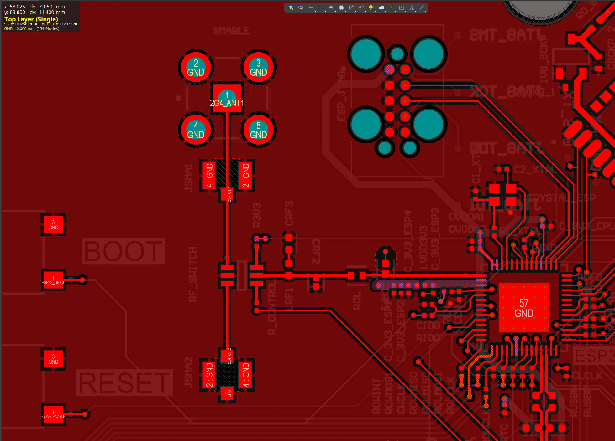
Layer Alternation to Identify Interfering Traces
With the RF region in focus, systematically toggle between layers to identify which signal traces pass directly beneath the RF trace. Begin with Layer 1 (Top), which contains the RF signal path itself. Then switch to Layer 2 (Mid-Layer 1) to observe the traces routed immediately beneath the RF region.
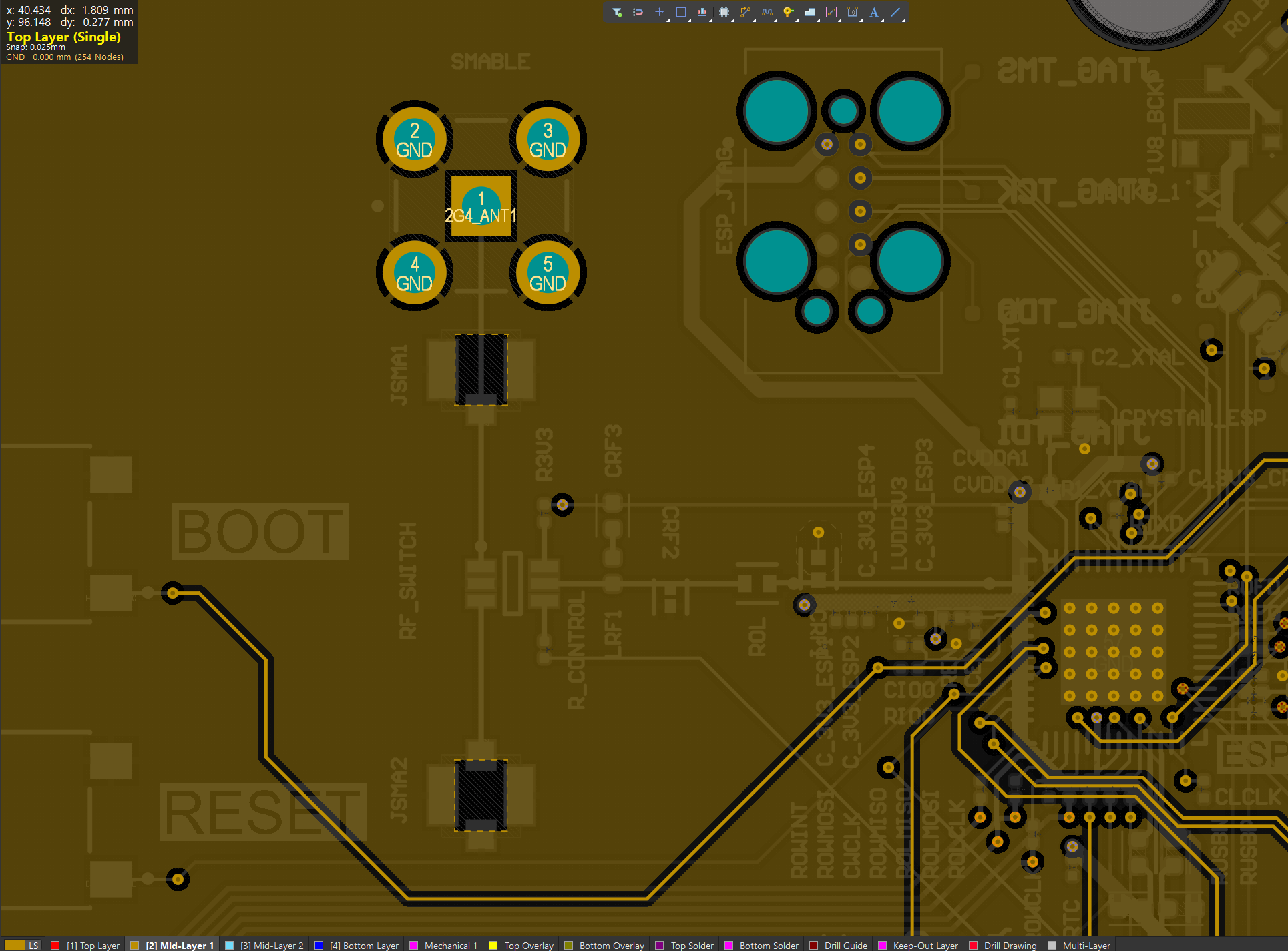
As the images will demonstrate, Layer 2 contains the boot trace line that passes directly under the RF circuit. This is the primary source of capacitive coupling identified in the previous section.
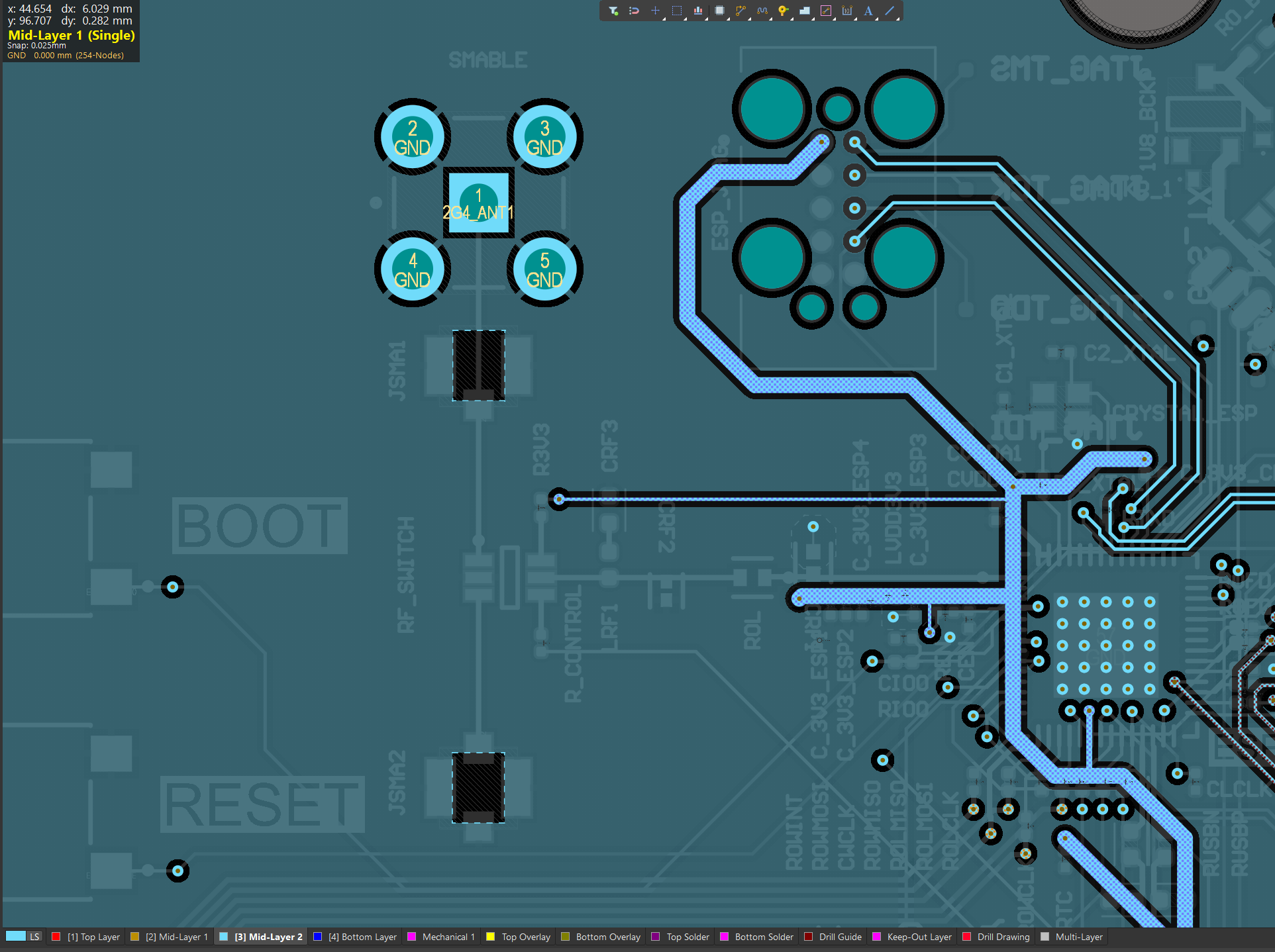
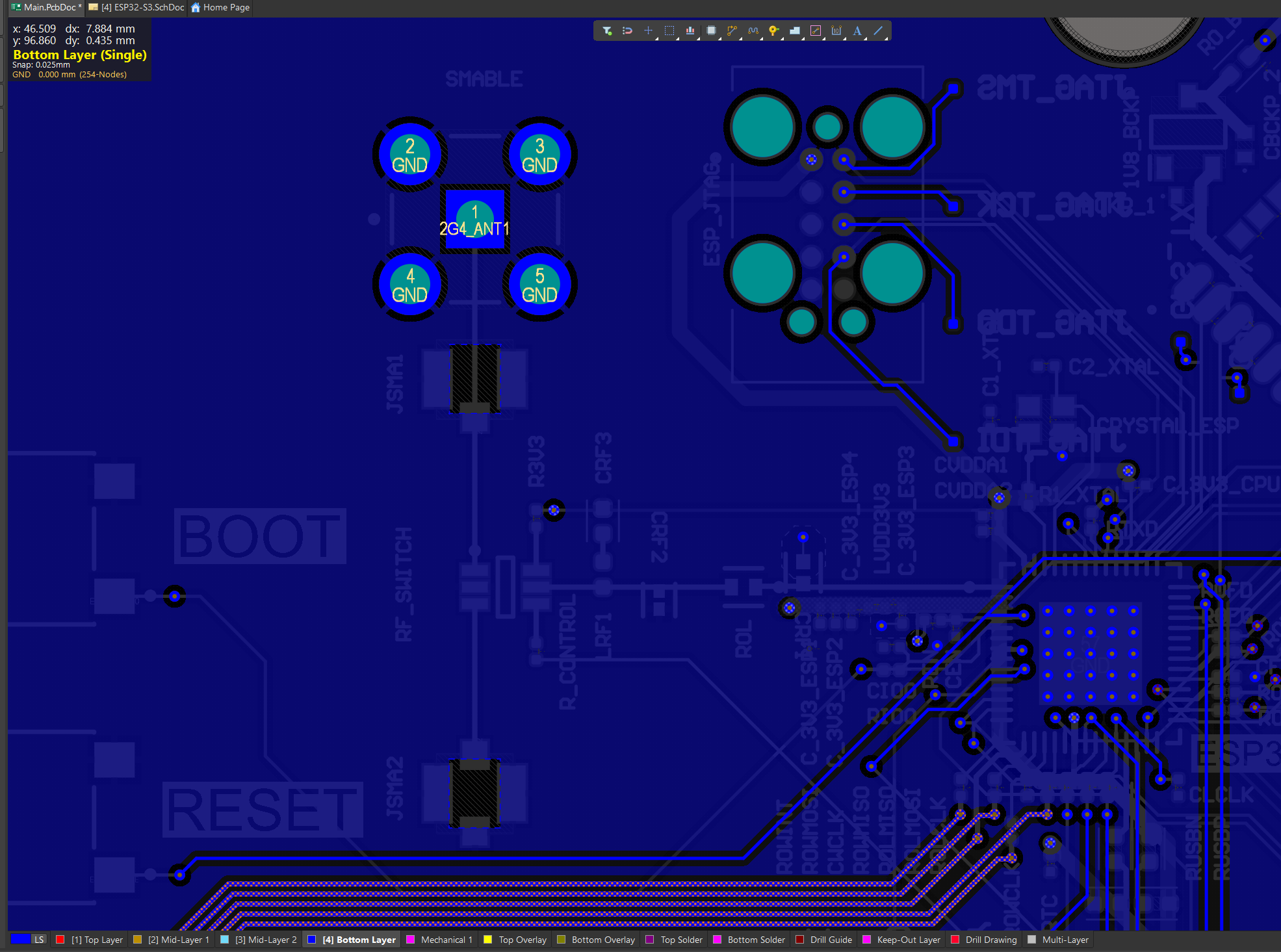
Continue to Layer 3 (Mid-Layer 2) and Layer 4 (Bottom) to assess the full coupling environment. Layer 3 contains the power distribution routing. Layer 4, being farthest from the RF trace, carries the digital reset path at a distance where coupling is negligible, but we still will address it.
Initiating Track Keepout Placement
With the interfering traces identified, begin the Track Keepout placement procedure. In Altium's toolbar, navigate to Place → Keepout → Solid Region. The cursor changes to a polygon drawing mode.
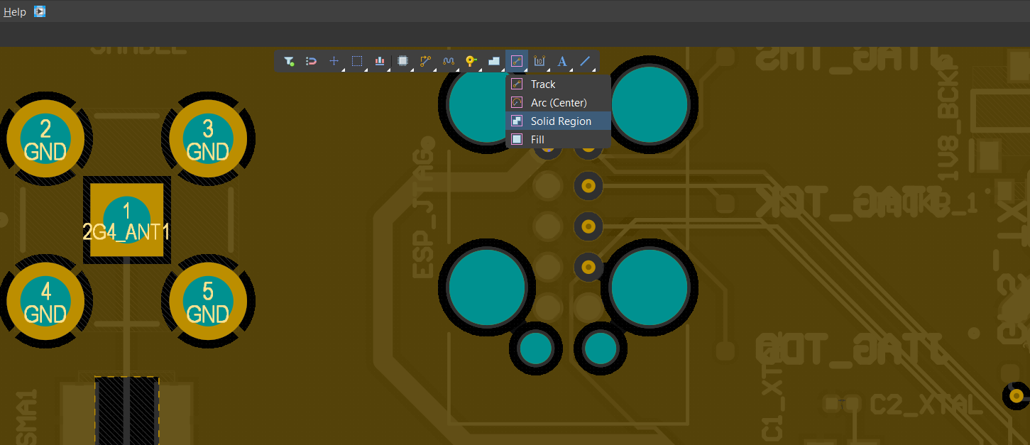
Click to define the vertices of a rectangular keepout polygon. The polygon should encompass the RF circuit and extend beyond it as a buffer.
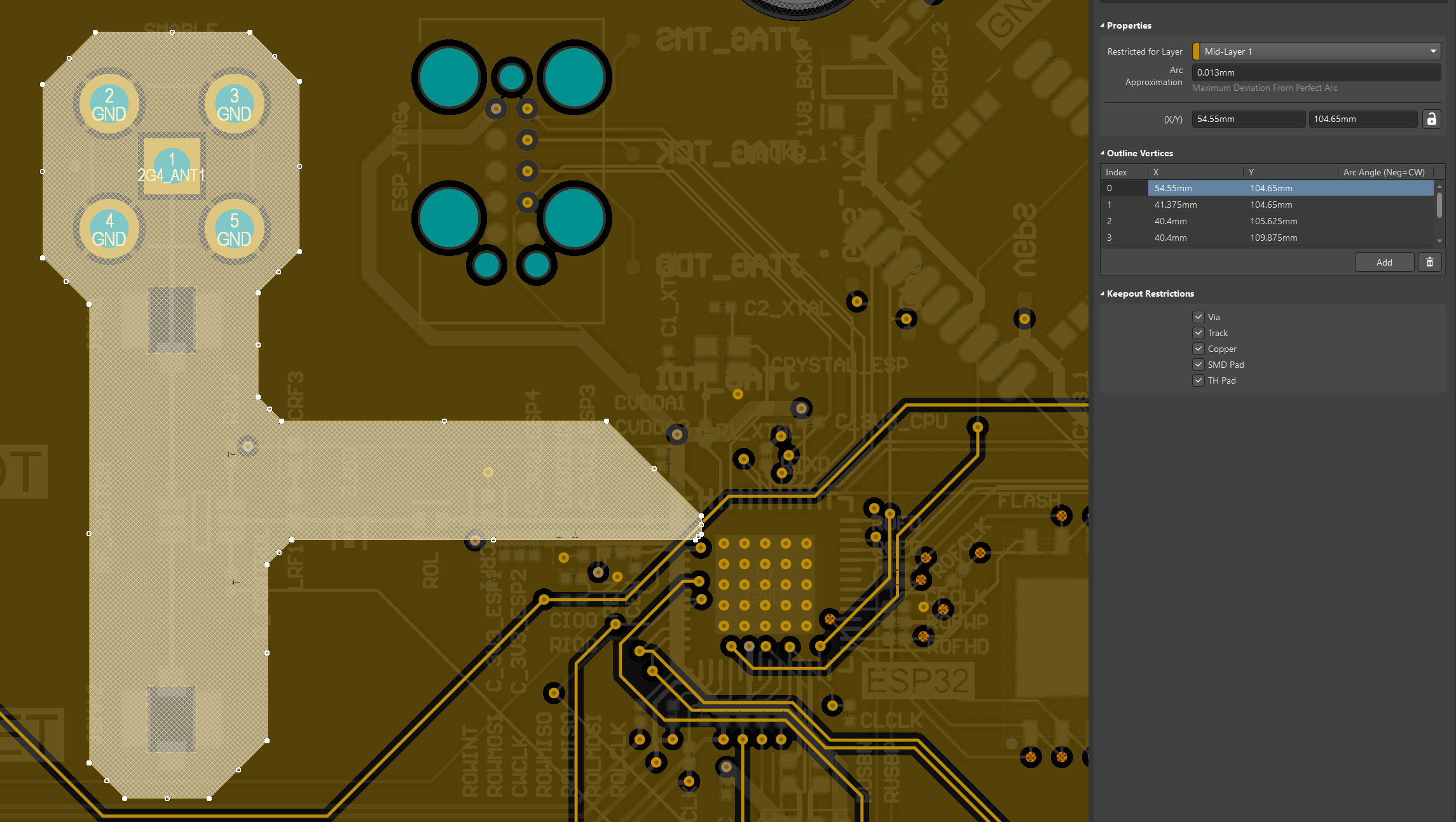
Configuring Keepout Restrictions
With the polygon placed, immediately select it and access its properties. A dialog box appears titled "Keepout Restrictions."

In this dialog, enable only the Track checkbox. Leave Via, Copper, SMD Pad, and TH Pad unchecked. This configuration allows ground stitching vias to pass through the exclusion zone while blocking signal traces.
Copying the Keepout Polygon to Other Layers
With the keepout polygon still selected on Layer 2, copy it using Ctrl+C. When prompted, select a fixed reference point, such as the center of the RF trace or a via next to the trace, to maintain precise geometric alignment.
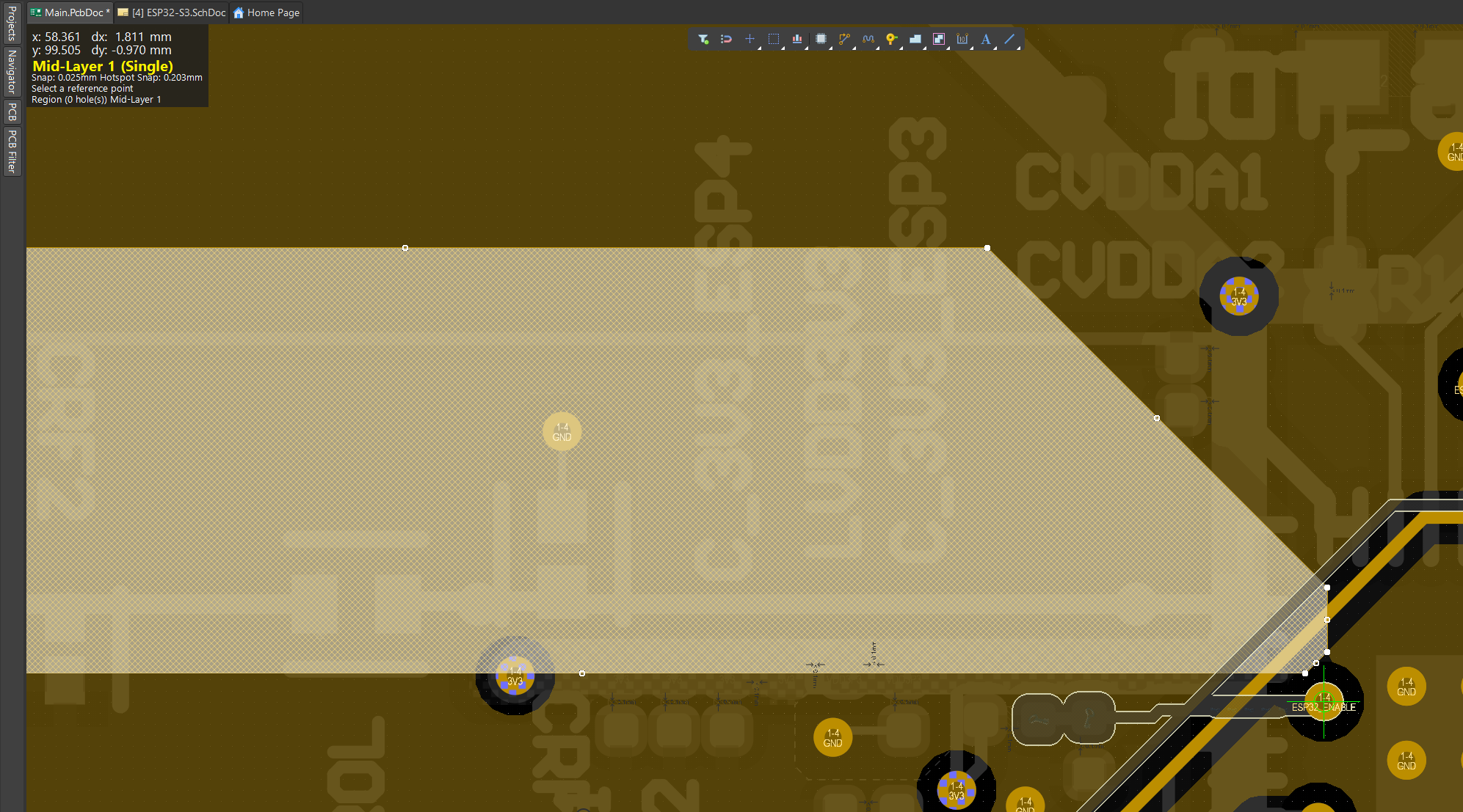
Paste the polygon in the second layer and change the polygon layer to layer 3.
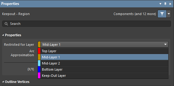
The polygon appears at the exact same X-Y coordinates on Layer 3, repeat the process to layer 4 (bottom).
Validation and Trace Repositioning
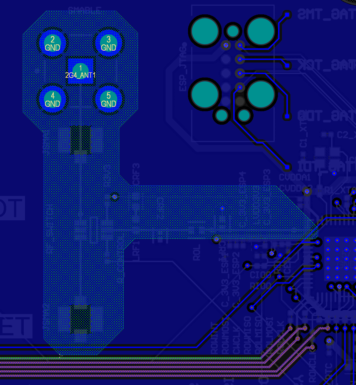
As you can see in the previous image, Altium is signaling errors on the keepout polygon, showing that there are violations to the polygon rule of not having any tracks passing through it. Iterate all layers containing the keepout polygon, addressing any violation by rerouting or pulling the traces to change their route.
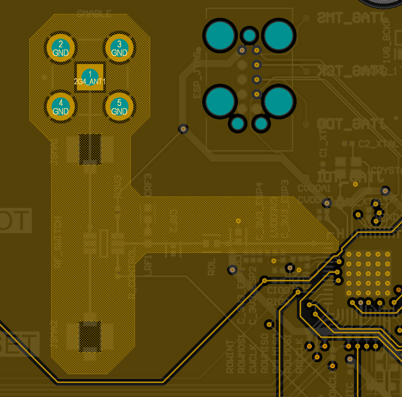
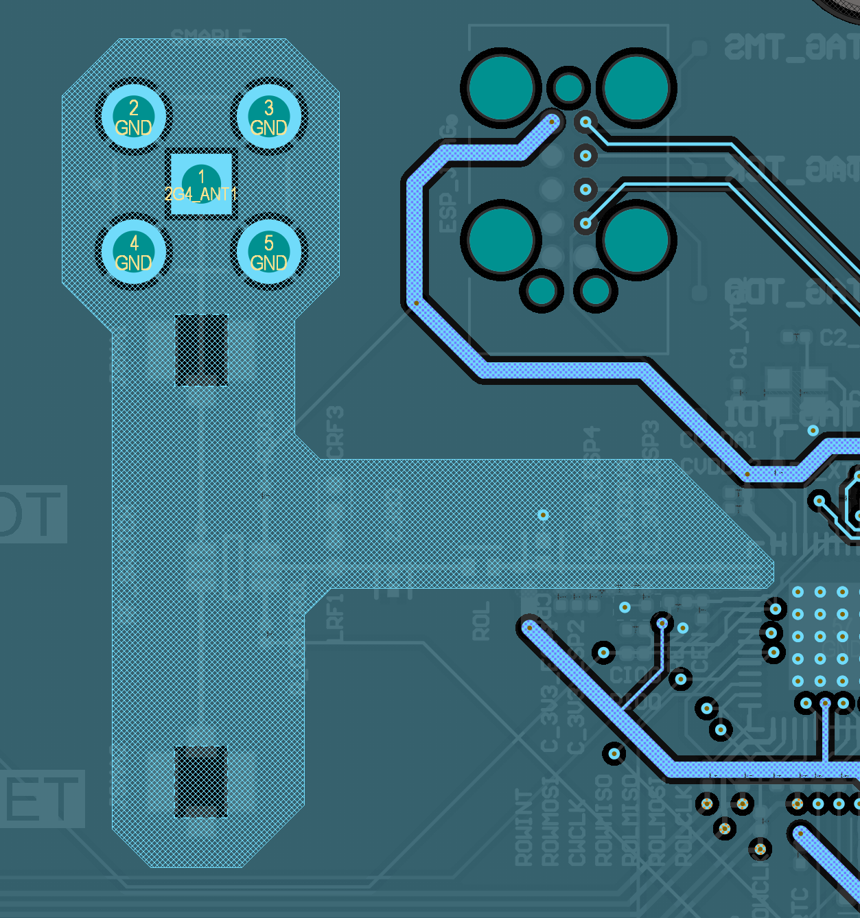
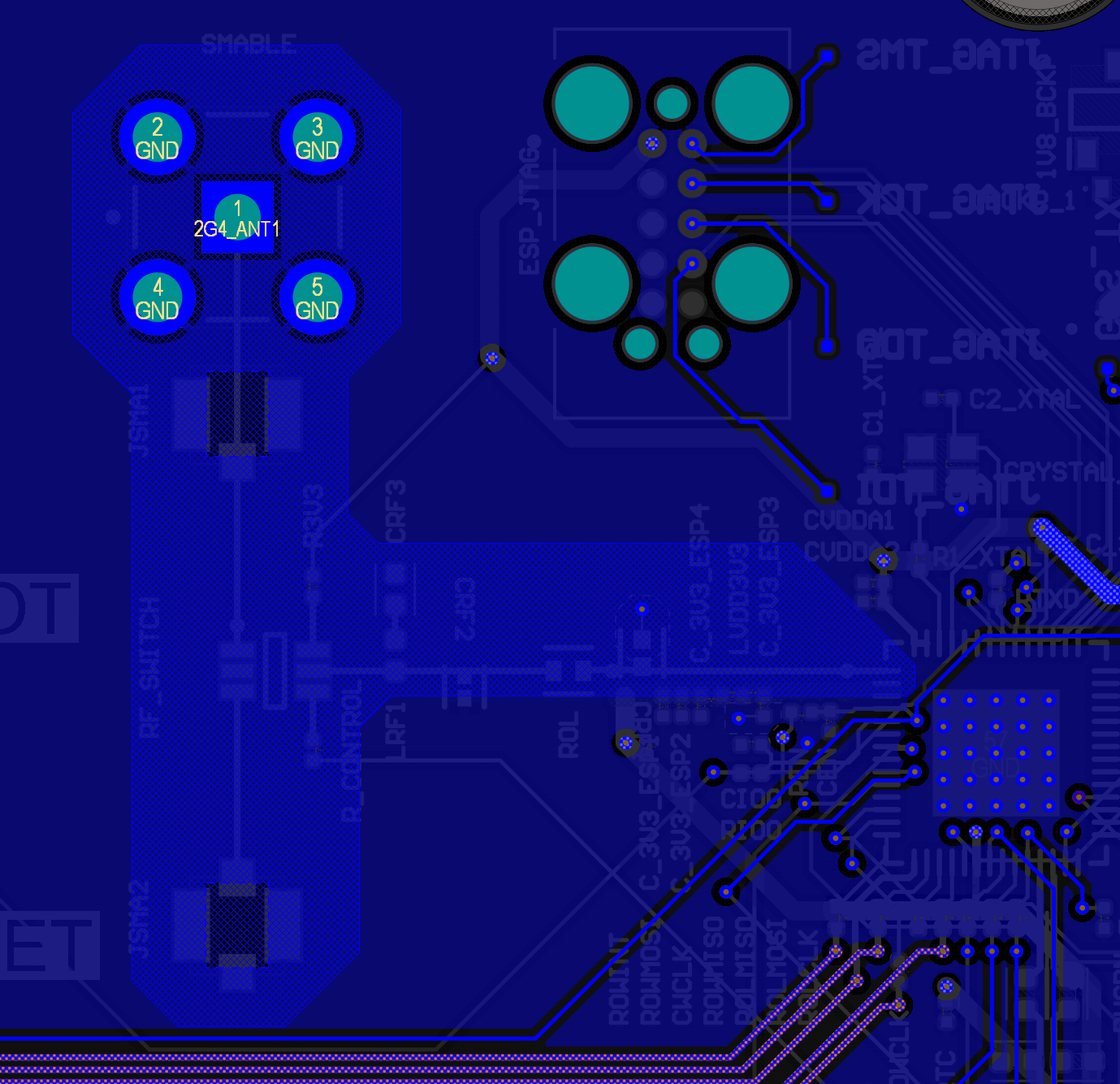
CST Studio Suite Re-Import and Co-Simulation Setup
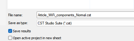
Open CST Studio Suite and load the baseline CST project from Article 3 (the one with the PCB layout already imported and optimized). Save this file with a clear suffix such as *_Baseline.cst or *_Original.cst. This becomes your reference, keep it open in a separate window.
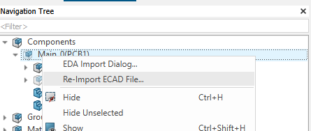
The Navigation Tree will show Components with the imported PCB listed. Right-click on the PCB entry and select Re-Import ECAD File. This refreshes the PCB geometry to reflect the modified layout.
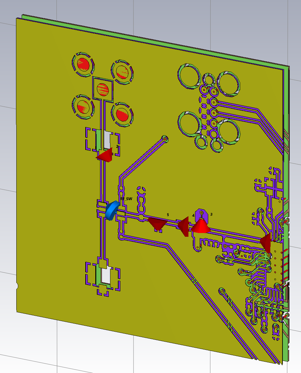
Since the geometry has changed, you will need to sweep around the components' values to find the optimal components for the new PCB, for this, save the project as a new file with “*_ports” suffix.

Change the Lumped Elements to Ports.
Run the simulation and reconnect the components to the ports.
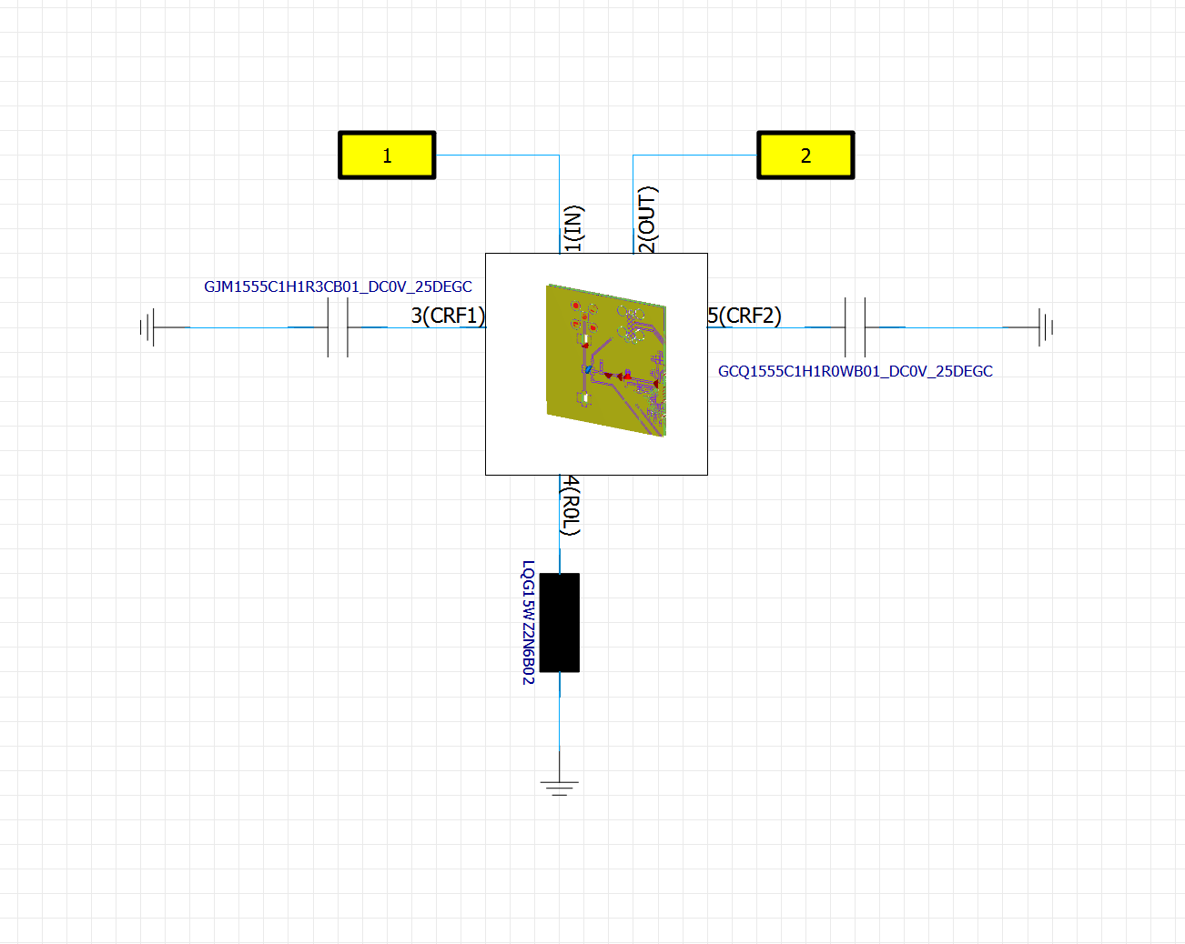
Use the ones you already downloaded or download new ones with the values near the original ones until you get a better match for the new geometry.
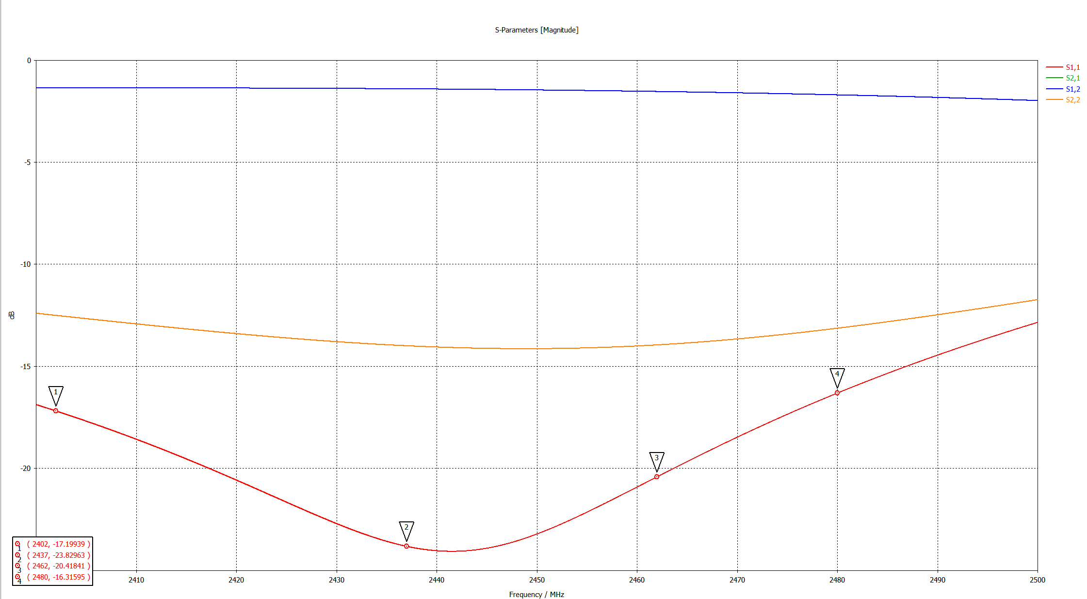
After this step, go back to the fixed components project and change them for the ones you found, keep them both showing using “Tile All” right-clicking the tab.
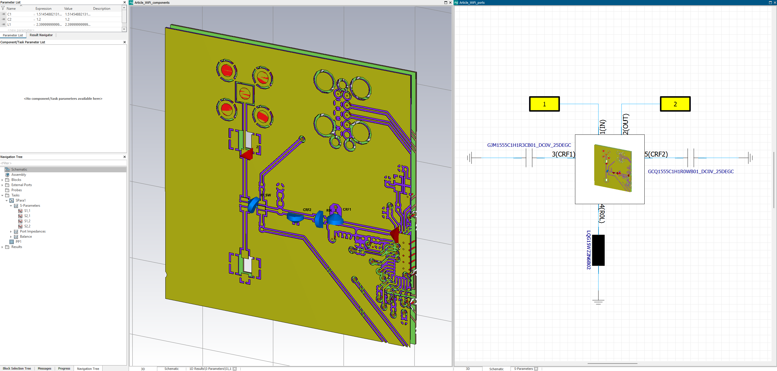
Update the simulation and get the new results with the fixed components, they won’t be the same but very similar.
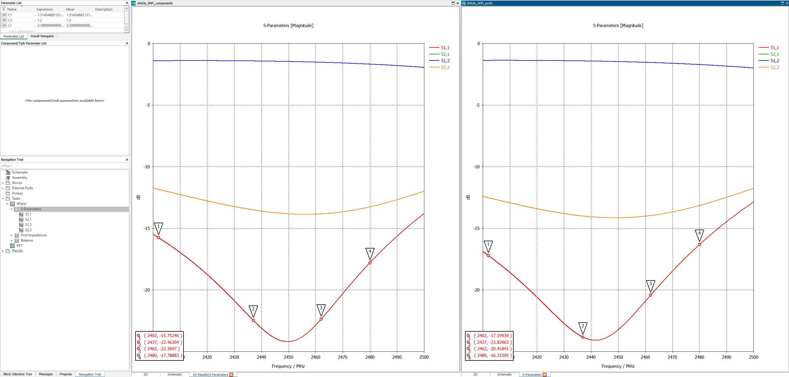
Results and Comparison
The Track Keepout implementation has been completed in Altium Designer. Three signal layers now contain Track Keepout polygons with proper restrictions configured. All DRC violations have been resolved, traces have been repositioned, and the modified PCB layout has been exported to ODB++ format and re-imported into CST Studio Suite.
Two parallel CST projects are now ready for comparison: the baseline project from Article 3 (without Track Keepout) and the new project with Track Keepout geometry implemented. Both projects use identical component models from Murata's catalog, ensuring that any differences in simulation results are attributable solely to the geometric changes introduced by the keepout zones.
The simulation has been executed on both projects, and S-parameter data has been extracted across the entire 2400–2500 MHz Wi-Fi band. The critical measurement is the S1,1 parameter, the return loss, at the four target frequencies: 2402, 2437, 2462, and 2480 MHz.
The results reveal the immediate electromagnetic consequence of the Track Keepout implementation.
S1,1 Comparison: Baseline vs. Track Keepout
At 2402 MHz, the baseline S1,1 is −15.31 dB. With Track Keepout implemented and no component re-optimization, S1,1 drops to −14.60 dB, a degradation of +0.71 dB. This represents a modest increase in reflection, but remains within acceptable bounds for Wi-Fi applications.
At 2437 MHz, the baseline is −22.15 dB, one of the best-matched points in the band. Track Keepout degrades this to −19.01 dB, a loss of +3.14 dB. At this frequency, the keepout's effect is more pronounced.
At 2462 MHz (the primary Wi-Fi data channel), the baseline achieves −26.34 dB, an exceptionally low reflection coefficient indicating near-perfect impedance matching. Track Keepout reduces this to −19.10 dB, a degradation of +7.24 dB. This is the most severe impact observed across the band.
At 2480 MHz, the baseline is −20.60 dB. Track Keepout degrades it to −16.32 dB, a loss of +4.28 dB.
Averaged across the four target frequencies, the Track Keepout implementation produces a mean S1,1 degradation of approximately +3.84 dB, a significant but not catastrophic shift. The variation across the band (from +0.71 dB to +7.24 dB) indicates that the keepout's effect is frequency-dependent, with the strongest impact near the center of the Wi-Fi band.
Physical Interpretation: Impedance Distortion
This degradation is not surprising. The Track Keepout removes signal traces from the region directly beneath the RF trace, eliminating the primary coupling path identified in the previous section. However, it does not change the fundamental stackup geometry, the dielectric thickness, ground plane structure, or trace dimensions remain unchanged.
What changes is the distributed capacitance seen by the RF trace at Layer 2. With interfering signal traces present, they form a distributed network of parallel conductors that couple to the RF path through the dielectric. Removing them eliminates this coupling source but also changes the electromagnetic boundary conditions surrounding the RF trace.
The RF circuit now "sees" a different characteristic impedance at its input. Instead of the ideal 35 Ω reference, the input impedance becomes frequency-dependent, varying with the spectral content of the nearby ground plane geometry and the remaining copper structure on Layer 3.
The S1,1 degradation reflects this impedance shift. At frequencies where the new impedance diverges most strongly from 35 Ω, the reflection is greatest. At 2462 MHz, where the baseline design had achieved exceptional matching (−26.34 dB), the degradation is most severe because the baseline relied on precise impedance matching in an environment with specific coupling characteristics, characteristics that the keepout has now altered.
Component Re-Optimization: Recovery Strategy
The degradation observed without component adjustment is the motivation for the re-optimization process documented in the Altium workflow. The three RF components (CRF1, CRF2, R0L) were originally tuned for an environment with interfering traces present on Layer 2. To restore performance in the new keepout environment, they must be re-tuned to compensate for the changed impedance boundary conditions.
Using Murata's SimSurfing tool and rapid CST co-simulation updates, alternative component values are tested systematically. The goal is to find component values that restore S1,1 matching to within ±0.3 dB of the baseline across all four target frequencies.
After component re-optimization, the results shift significantly. At 2402 MHz, S1,1 improves from −14.60 dB to −15.75 dB, now +0.44 dB relative to baseline, within specification. At 2437 MHz, it recovers to −22.46 dB, only −0.32 dB better than baseline, a remarkable achievement indicating that the optimized design actually exceeds baseline performance at this frequency.
At 2462 MHz, the re-optimized design achieves −22.37 dB. While this represents a +3.97 dB degradation relative to the baseline's exceptional −26.34 dB, it is still a respectable S1,1 value in absolute terms (reflection magnitude of approximately −22 dB corresponds to a return loss of 22 dB, well-matched by industry standards).
At 2480 MHz, the optimized result is −17.79 dB, a +2.81 dB degradation from baseline but still within the acceptable range for Wi-Fi operation.
Across all four frequencies, the optimized Track Keepout design has recovered approximately 51% of the initial S1,1 degradation. More importantly, at 2402 and 2437 MHz, it actually achieves performance superior to the baseline, a result that validates the re-optimization process and demonstrates that the keepout environment, when properly compensated, can yield excellent RF matching.
Trade-offs and Design Implications
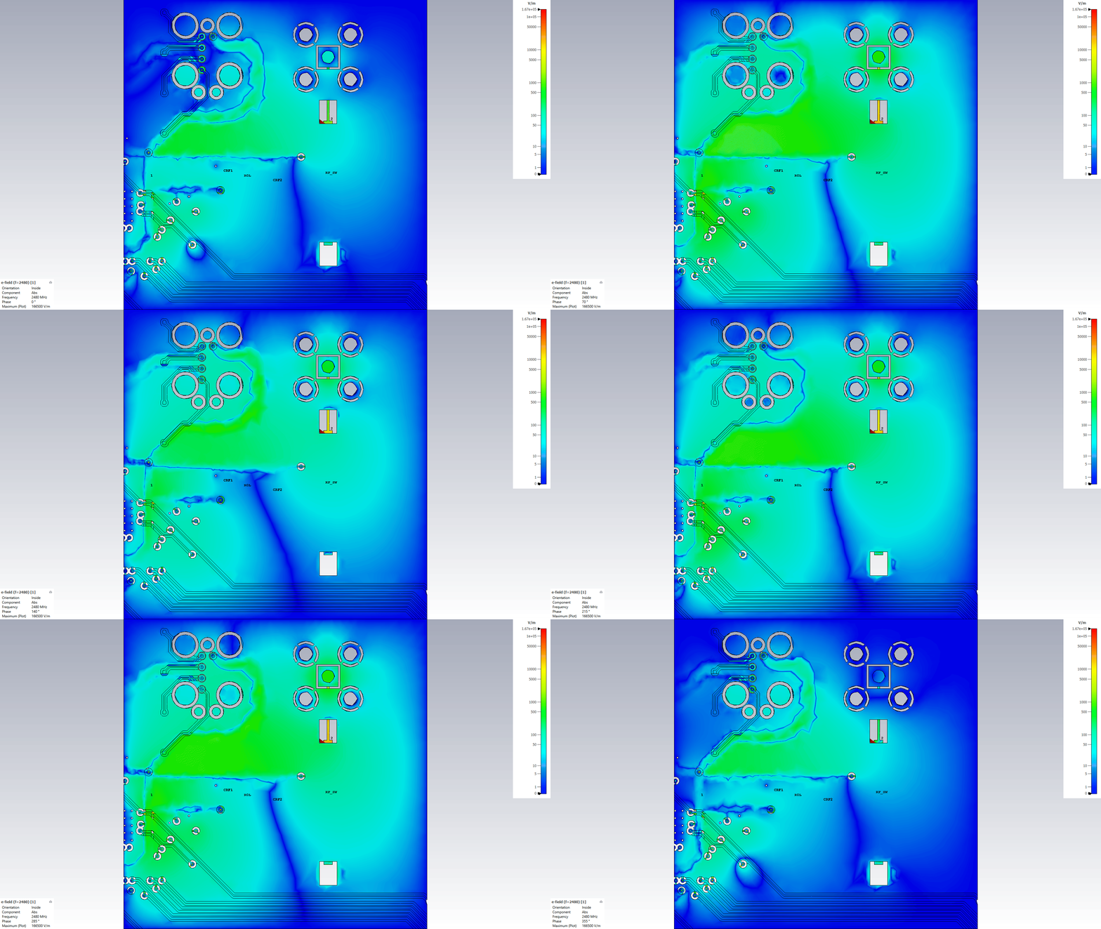
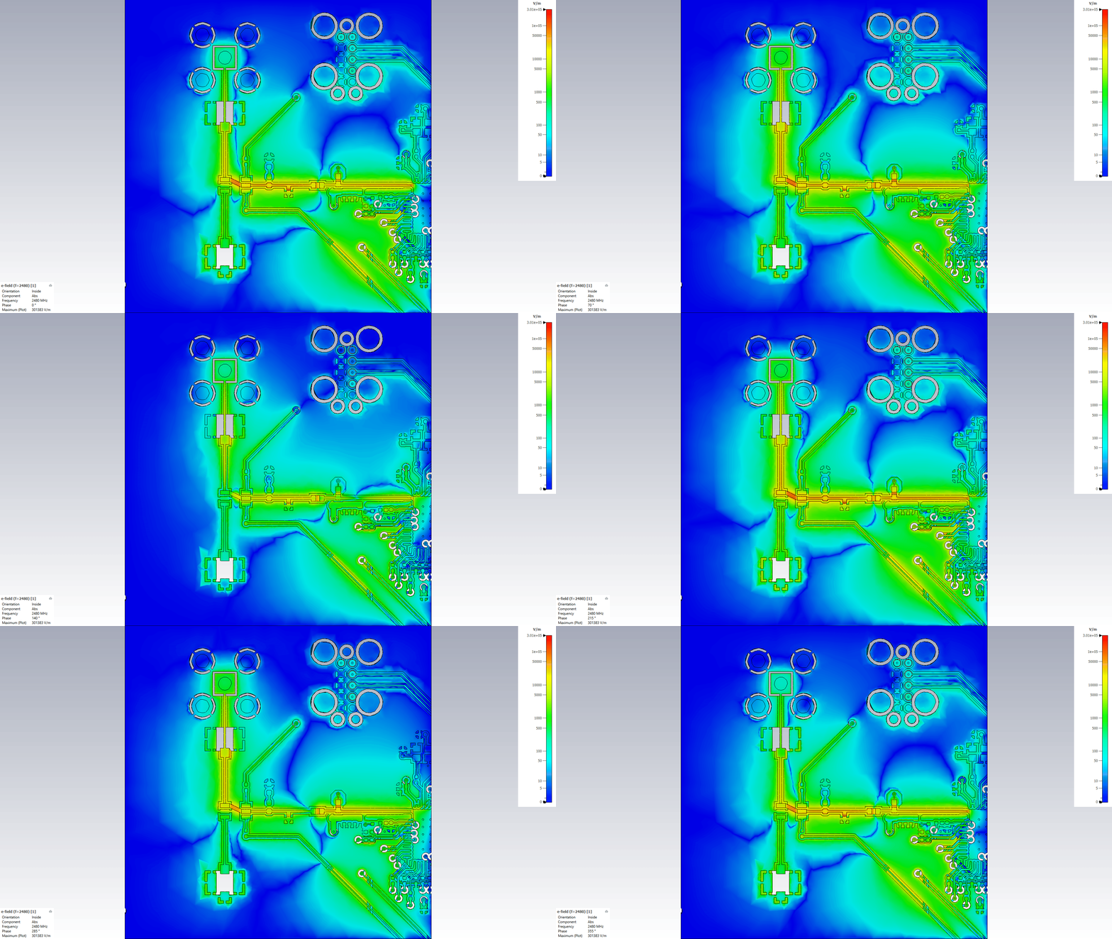
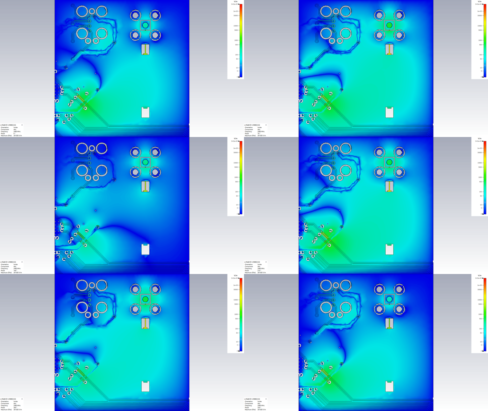
The Track Keepout technique successfully isolates the RF circuit from signal traces on internal layers. The benefit is quantifiable in electromagnetic field visualizations (to be presented in subsequent articles): E-field leakage to Layer 2 is substantially reduced, lateral magnetic field extension is confined, and surface currents distribute less widely into adjacent copper regions.
The cost is a change in impedance boundary conditions that requires component re-optimization. This is not a deficiency of the technique but rather a natural consequence of modifying the electromagnetic environment in which the RF circuit operates.
The trade-off is favorable. Complete electromagnetic isolation cannot be achieved without moving to a different PCB architecture (dedicated RF layers, shielding cans, or more sophisticated layer arrangements). Within the constraints of a four-layer, cost-optimized design, Track Keepout offers substantial isolation benefits with manageable cost in performance recovery.
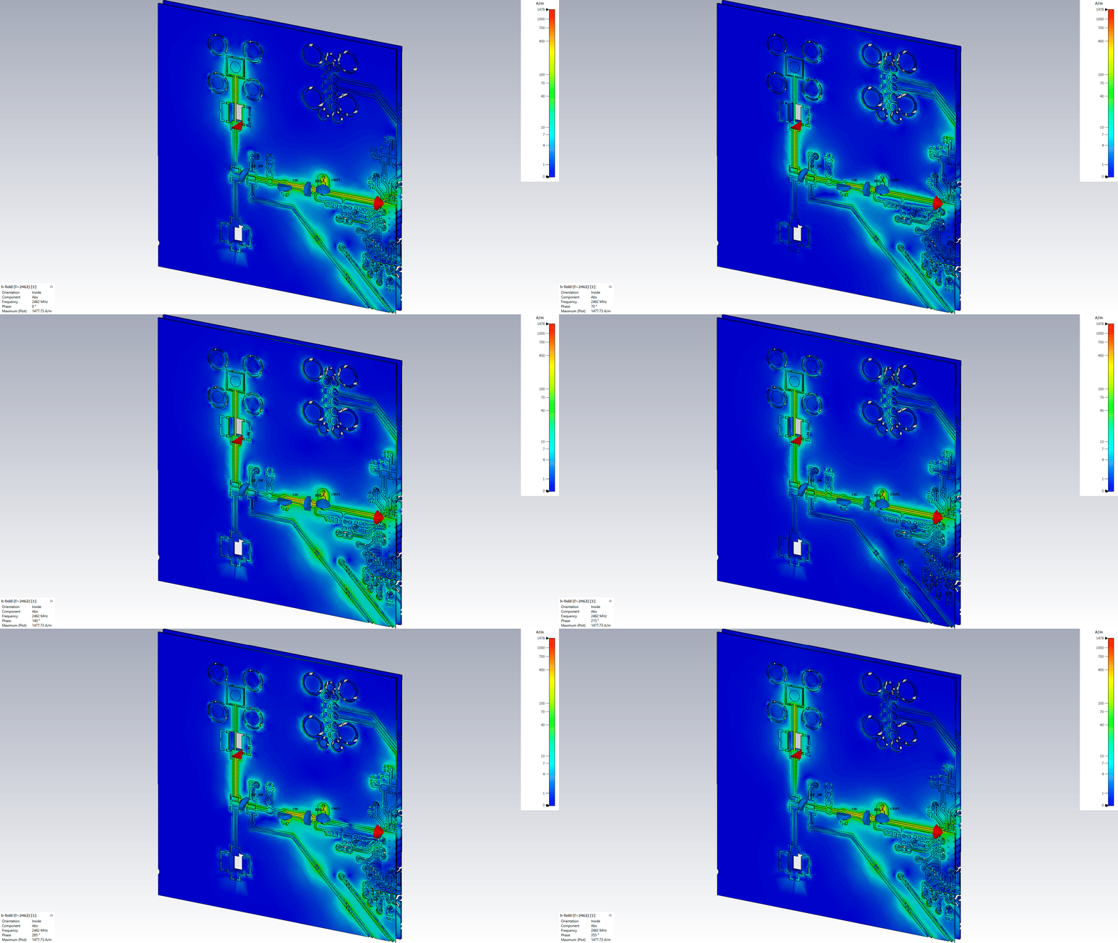
Simulation results
Original:
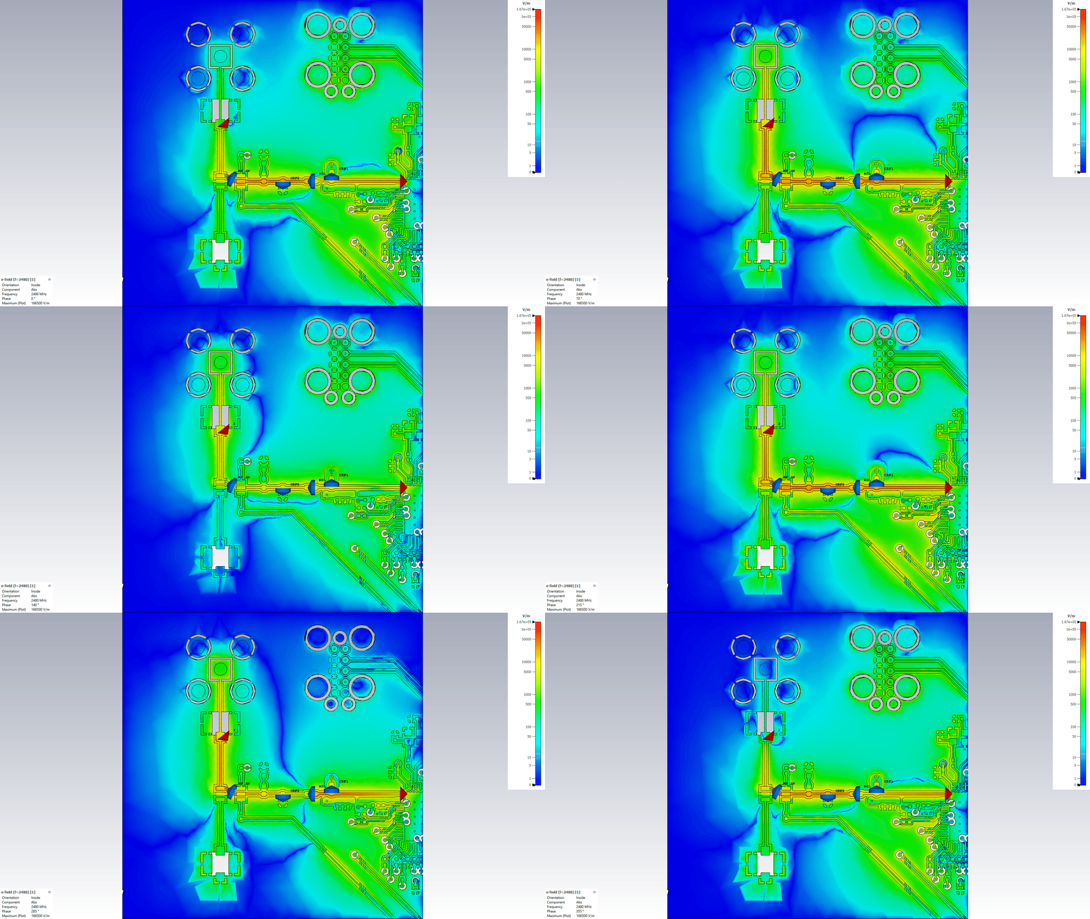
Optimized + Keepout:
Conclusion and Next Steps
Article 4 has documented the design, implementation, and initial validation of Track Keepout polygons for RF crosstalk isolation in a four-layer PCB. The technique is practical, implementable within existing CAD tools, and produces measurable electromagnetic benefits without requiring stackup redesign.
The key findings are:
Track Keepout is effective for passive isolation of the reference plane. Removing interfering signal traces from Layer 2 (the reference plane beneath the RF circuit) reduces crosstalk coupling and provides clear electromagnetic containment at the primary coupling interface.
Component re-optimization is essential. The changed impedance environment requires adjustment of the RF filter components. Using Murata's SimSurfing tool and rapid CST iteration, acceptable performance can be recovered across the Wi-Fi band.
Trade-offs are manageable. The cost in S-parameter degradation (3–4 dB at mid-band frequencies) is recoverable through component selection, and the benefit in electromagnetic confinement justifies the effort.
Integration with additional techniques is necessary for complete isolation. Track Keepout alone addresses the primary path but does not fully contain secondary coupling modes. Via stitching (Article 5) extends confinement by creating a boundary on the reference plane itself, and ground plane cutout (Article 6) addresses resonant modes within the reference plane structure. Together, the three techniques create a complete isolation strategy.
The workflow established in this article, PCB layout modification in Altium, re-import and re-simulation in CST, component iteration using Murata datasheets, and quantitative S-parameter comparison, is scalable and applicable to any RF circuit on a multilayer PCB facing similar crosstalk challenges.
Article 5 will extend this methodology by adding via stitching around the RF region, documenting its electromagnetic effects on the reference plane confinement, and demonstrating how to integrate it with Track Keepout for enhanced isolation. The cumulative knowledge across Articles 4, 5, and 6 will provide a complete design methodology for EMI mitigation in compact RF systems through coordinated control of the reference plane layer.